My most re-used Python code for A/B testing
Import the things you need
from matplotlib import pyplot as plt
import pandas as pd
import numpy as np
from scipy  import norm, stats, binom, mannwhitneyu
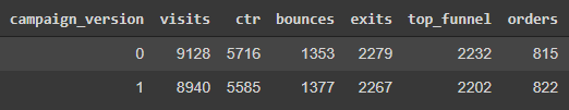
There are a few ways the data could be set up. Step 1 is viewing the data you have, using the dataframe name like test_data or the .head() method. test_data.head() will give you something like the below:
Once you have the test data you want to make sure the split was accurate. To do that run a sample ratio mismatch test on the users/visitors/sessions data. Below uses .iloc[] and .sum() to insert the visits data.
stats.binom_test(test_data.iloc[1,1], test_data['visits'].sum(), 0.5)
0.16416588441261487
Another method that I use for other calculations just pulls the appropriate cell. That is shown below:
stats.binom_test((test_data[test_data.campaign == '1'].visits), test_data['visits'].sum(), 0.5)
0.16416588441261487
The difference from .iloc[] and (test_data[test_data.campaign == '1'].visits), is that this is saying in the test_data, where the campaign_version is equal to 1, return that visit number. This to me is easier than .iloc because I don’t have to worry about the dataframe location being wrong or changing. And you can see both approaches return the same number.
I typically look for anything less than 0.05 or 0.01. If you find SRM you need to look into why this could be the case since any results are not valid. Here’s a helpful link of probable causes and some things to look into.
If there’s no, SRM you can go on to comparing the metrics.
To look at rates instead of raw numbers to get a better sense of the data I use the following approach:
dataframe['new_metric'] = dataframe.column1 {/*+-} dataframe.column2
test_data['ctr_rate'] = test_data.ctr/test_data.visits
test_data['bounce_rate'] = test_data.bounces/test_data.visits
test_data['exit_rate'] = test_data.exits/test_data.visits
test_data['atc_rate'] = test_data.top_funnel/test_data.visits
test_data['cvr'] = test_data.orders/test_data.visits
test_data['bof'] = test_data.orders/test_data.top_funnel
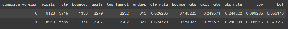
test_data
The table now has 6 additional columns of rates based off the data.
While not entirely necessary, the rates are helpful to see from a high level. It also helps set up the graphs. I’m going to store the rates I want to examine as variables to help in calculations going forward.
cont_visits, test_visits = float(test_data[test_data.campaign_version == '0'].visits), float(test_data[test_data.campaign_version == '1'].visits)

cont_atc, test_atc = float(test_data[test_data.campaign_version == '0'].top_funnel), float(test_data[test_data.campaign_version == '1'].top_funnel)

cont_rate, test_rate = cont_atc / cont_visits, test_atc / test_visits
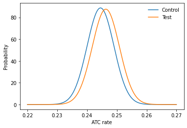
I’m starting by looking at the top_funnel or add to cart metric. You can do the same for any other metric. The calculations and graphs need our visit number, ATC number, and ATC rate for each variation. (Using the float() saves them as numbers we can use vs just calling them).
# Calculate standard deviation performance and plot.
std_cont = np.sqrt(cont_rate * (1 - cont_rate) / cont_visits)
std_test = np.sqrt(test_rate * (1 - test_rate) / test_visits)

click_rate = np.linspace(0.22, 0.27, 200)
prob_a = norm(cont_rate, std_cont).pdf(click_rate)
prob_b = norm(test_rate, std_test).pdf(click_rate)

# Make the bar plots.
plt.plot(click_rate, prob_a, label="Control")
plt.plot(click_rate, prob_b, label="Test")
plt.legend(frameon=False)
plt.xlabel("ATC rate");
plt.ylabel("Probability");
z_score = (test_rate - cont_rate) / np.sqrt(std_cont**2 + std_test**2)
p = norm(test_rate - cont_rate, np.sqrt(std_cont**2 + std_test**2))
x = np.linspace(-0.03, 0.04, 1000)
y = p.pdf(x)
area_under_curve = p.sf(0)
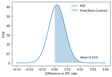
plt.plot(x, y, label="PDF")
plt.fill_between(x, 0, y, where=x>0, label="Prob(Test>Control)", alpha=0.3)
plt.annotate(f"Area={area_under_curve:0.3f}", (0.02, 5))
plt.legend()
plt.xlabel("Difference in ATC rate"); plt.ylabel("Prob");
diff = round(test_rate - cont_rate,4)
print("Change in ATC is", diff*100,"%")
print(f"zscore is {z_score:0.3f}, with p-value {norm().sf(z_score):0.3f}")
Change in ATC is 0.18 %
zscore is 0.279, with p-value 0.390
Just checking my work and looking at the confidence intervals:
def get_z_score(alpha):
    return norm.ppf(alpha)

alpha = 0.05
import math as mt

pool = (test_data.top_funnel.sum()/test_data.visits.sum())
p_sd = mt.sqrt(pool*(1-pool)*(1/cont_visits + 1/test_visits))
z = (test_rate - cont_rate)/p_sd
me = round(get_z_score(1-alpha/2)*p_sd,4)
diff = (test_rate - cont_rate)

print("Change in ATC is", diff*100,"%")
print("Confidence interval: [", diff-me, ",", diff+me, "]")

Change in ATC is 0.17863760153874197 % Confidence interval: [ -0.01081362398461258 , 0.01438637601538742 ]
The difference in the ATC rate matches and the confidence intervals show -1% to +1% which is what I’d expect to see.
At this time, no statistical difference is detected from the changes we made.